21  Analyseren: topic modeling

library(topicmodels)

rv_dtm <- tidytext_woord %>% 
  group_by(bestandsnaam, text) %>% 
  summarise(aantal = n()) %>% 
  cast_dtm(term = text, document = bestandsnaam, value = aantal)
`summarise()` has grouped output by 'bestandsnaam'. You can override using the
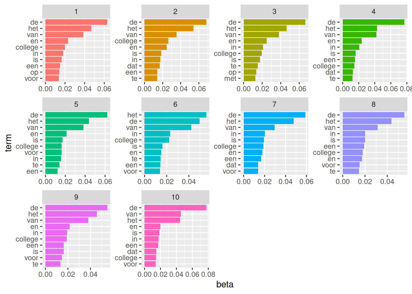
`.groups` argument.
rv_lda <- LDA(rv_dtm, k = 10, control = list(seed = 1234))
rv_topics <- tidy(rv_lda, matrix = "beta")
rv_topics
# A tibble: 139,230 × 3
   topic term     beta
   <int> <chr>   <dbl>
 1     1 1     0.00635
 2     2 1     0.00268
 3     3 1     0.00556
 4     4 1     0.00397
 5     5 1     0.00797
 6     6 1     0.0112 
 7     7 1     0.00225
 8     8 1     0.00729
 9     9 1     0.00966
10    10 1     0.00430
# ℹ 139,220 more rows
rv_top_terms <- rv_topics %>% 
  group_by(topic) %>% 
  slice_max(beta, n = 10) %>% 
  ungroup() %>% 
  arrange(topic, -beta)

rv_top_terms %>% 
  mutate(term = reorder_within(term, beta, topic)) %>%
  ggplot(aes(beta, term, fill = factor(topic))) +
  geom_col(show.legend = FALSE) +
  facet_wrap(~ topic, scales = "free") +
  scale_y_reordered()